Note
Using the DLRUTDataset#
This example shall give an overview of the methods and attributes that are available in the DLRUTDataset class.
Load trajectory data#
At first, we need to load the trajectory data of the dataset.
[1]:
from tasi.dlr.dataset import DLRTrajectoryDataset, DLRUTDatasetManager, DLRUTVersion
from tasi.tests import DATA_PATH

dataset = DLRUTDatasetManager(DLRUTVersion.v1_2_0, path=DATA_PATH)
dataset.load()

ds = DLRTrajectoryDataset.from_csv(dataset.trajectory()[0])
Extracting: 100%|██████████| 16/16 [00:00<00:00, 38.04file/s]
Attributes of the dataset#
There are several attributes available to get information about a dataset. For instance, we can get the interval of a dataset via the property
[2]:
ds.interval
[2]:
Interval(2023-09-24 12:00:00.016482+00:00, 2023-09-24 12:14:59.966482+00:00, closed='right')
or all unique timestamps of it via
[3]:
ds.timestamps
[3]:
DatetimeIndex(['2023-09-24 12:00:00.016482+00:00',
               '2023-09-24 12:00:00.066482+00:00',
               '2023-09-24 12:00:00.116482+00:00',
               '2023-09-24 12:00:00.166482+00:00',
               '2023-09-24 12:00:00.216482+00:00',
               '2023-09-24 12:00:00.266482+00:00',
               '2023-09-24 12:00:00.316482+00:00',
               '2023-09-24 12:00:00.366482+00:00',
               '2023-09-24 12:00:00.416482+00:00',
               '2023-09-24 12:00:00.466482+00:00',
               ...
               '2023-09-24 12:14:59.516482+00:00',
               '2023-09-24 12:14:59.566482+00:00',
               '2023-09-24 12:14:59.616482+00:00',
               '2023-09-24 12:14:59.666482+00:00',
               '2023-09-24 12:14:59.716482+00:00',
               '2023-09-24 12:14:59.766482+00:00',
               '2023-09-24 12:14:59.816482+00:00',
               '2023-09-24 12:14:59.866482+00:00',
               '2023-09-24 12:14:59.916482+00:00',
               '2023-09-24 12:14:59.966482+00:00'],
              dtype='datetime64[ns, UTC]', name='timestamp', length=18000, freq=None)
or the ids of all traffic participants in the dataset.
[4]:
ds.ids
[4]:
Index([1695556712692966, 1695556715491157, 1695556722944961, 1695556743992329,
       1695556773745982, 1695556777842612, 1695556779393896, 1695556779791865,
       1695556783142714, 1695556784842671,
       ...
       1695557692745846, 1695557694242959, 1695557693443711, 1695557695048101,
       1695557694145046, 1695557695944822, 1695557698396270, 1695557698694887,
       1695557699646115, 1695557700093347],
      dtype='int64', name='id', length=636)
Filtering#
If you want to look into a short sequence of the overall dataset, you can select specific rows of the overall dataset. The tasi.DLRTrajectoryDataset provides various ways for this purpose.
Time and object#
There are two variants to filter a dataset based on the information on the dataset’s index. For instance, if you want to filter the dataset by an interval, you can utilize the tasi.DLRTrajectoryDataset.during method.
[5]:
ds.during(ds.timestamps[0], ds.timestamps[10])
[5]:
| acceleration | position | classifications | dimension | interpolated | velocity | yaw | ||||||||||||||
|---|---|---|---|---|---|---|---|---|---|---|---|---|---|---|---|---|---|---|---|---|
| easting | magnitude | northing | easting | northing | bicycle | car | motorbike | pedestrian | truck | van | height | length | width | easting | magnitude | northing | ||||
| timestamp | id | |||||||||||||||||||
| 2023-09-24 12:00:00.016482+00:00 | 1695556712692966 | 0.003 | 0.010 | 0.009 | 604755.977 | 5.793e+06 | 0.025 | 0.824 | 0.150 | 0.000 | 0.000 | 0.0 | 1.625 | 2.407 | 1.334 | False | 0.004 | 0.020 | 0.019 | -73.593 |
| 1695556715491157 | -1.093 | 1.235 | -0.575 | 604795.259 | 5.793e+06 | 0.000 | 0.883 | 0.109 | 0.005 | 0.003 | 0.0 | 1.556 | 3.463 | 2.045 | False | -3.971 | 4.113 | -1.074 | -164.869 | |
| 1695556722944961 | -0.000 | 0.001 | 0.001 | 604753.090 | 5.793e+06 | 0.000 | 0.579 | 0.334 | 0.000 | 0.087 | 0.0 | 1.682 | 2.135 | 1.124 | False | -0.000 | 0.008 | -0.008 | -69.165 | |
| 1695556743992329 | -0.005 | 0.007 | 0.006 | 604751.898 | 5.793e+06 | 0.000 | 0.590 | 0.060 | 0.000 | 0.344 | 0.0 | 1.990 | 2.508 | 1.565 | False | -0.012 | 0.016 | 0.010 | -68.221 | |
| 1695556773745982 | 0.013 | 0.021 | 0.016 | 604793.176 | 5.793e+06 | 0.002 | 0.811 | 0.176 | 0.011 | 0.000 | 0.0 | 1.366 | 2.739 | 1.101 | False | 0.014 | 0.026 | -0.022 | 110.513 | |
| ... | ... | ... | ... | ... | ... | ... | ... | ... | ... | ... | ... | ... | ... | ... | ... | ... | ... | ... | ... | ... |
| 2023-09-24 12:00:00.466482+00:00 | 1695556788746534 | 0.141 | 0.437 | -0.414 | 604792.629 | 5.793e+06 | 0.010 | 0.805 | 0.185 | 0.000 | 0.000 | 0.0 | 1.413 | 3.156 | 1.331 | False | -0.718 | 2.604 | 2.503 | 106.020 |
| 1695556791347026 | 1.090 | 1.096 | 0.117 | 604726.328 | 5.793e+06 | 0.022 | 0.850 | 0.127 | 0.001 | 0.000 | 0.0 | 1.341 | 2.560 | 1.478 | False | -12.970 | 13.190 | -2.395 | -169.489 | |
| 1695556796543589 | -0.288 | 0.996 | 0.954 | 604745.975 | 5.793e+06 | 0.000 | 0.956 | 0.039 | 0.000 | 0.000 | 0.0 | 1.431 | 3.562 | 1.607 | False | 1.310 | 4.049 | -3.831 | -71.134 | |
| 1695556796949041 | -0.025 | 0.080 | -0.076 | 604798.825 | 5.793e+06 | 0.000 | 0.530 | 0.292 | 0.000 | 0.000 | 0.0 | 1.619 | 2.723 | 1.308 | False | -0.483 | 2.839 | 2.797 | 99.775 | |
| 1695556798142269 | -0.526 | 0.546 | 0.147 | 604800.375 | 5.793e+06 | 0.000 | 0.986 | 0.001 | 0.007 | 0.006 | 0.0 | 1.315 | 3.602 | 1.776 | False | -14.831 | 15.541 | -4.643 | -162.637 | |
170 rows × 19 columns
that returns the rows within the given interval.
Another variant to select specific rows of the datasets is by the id of a traffic participant. This might be useful if you want to take a closer look into the behavior of specific traffic participants. For instance, to filter by the second traffic participant in the dataset, we can combine the tasi.DLRTrajectoryDataset.ids attribute with the trajectory method.
[6]:
ds.trajectory(ds.ids[1])
[6]:
| acceleration | position | classifications | dimension | interpolated | velocity | yaw | ||||||||||||||
|---|---|---|---|---|---|---|---|---|---|---|---|---|---|---|---|---|---|---|---|---|
| easting | magnitude | northing | easting | northing | bicycle | car | motorbike | pedestrian | truck | van | height | length | width | easting | magnitude | northing | ||||
| timestamp | id | |||||||||||||||||||
| 2023-09-24 12:00:00.016482+00:00 | 1695556715491157 | -1.093 | 1.235 | -0.575 | 604795.259 | 5.793e+06 | 0.0 | 0.883 | 0.109 | 0.005 | 0.003 | 0.0 | 1.556 | 3.463 | 2.045 | False | -3.971 | 4.113 | -1.074 | -164.869 |
| 2023-09-24 12:00:00.066482+00:00 | 1695556715491157 | -1.075 | 1.223 | -0.583 | 604795.043 | 5.793e+06 | 0.0 | 0.883 | 0.109 | 0.005 | 0.003 | 0.0 | 1.556 | 3.463 | 2.045 | False | -4.042 | 4.189 | -1.099 | -164.781 |
| 2023-09-24 12:00:00.116482+00:00 | 1695556715491157 | -1.057 | 1.212 | -0.591 | 604794.824 | 5.793e+06 | 0.0 | 0.883 | 0.109 | 0.005 | 0.003 | 0.0 | 1.556 | 3.463 | 2.045 | False | -4.111 | 4.262 | -1.126 | -164.688 |
| 2023-09-24 12:00:00.166482+00:00 | 1695556715491157 | -1.039 | 1.199 | -0.600 | 604794.601 | 5.793e+06 | 0.0 | 0.883 | 0.109 | 0.005 | 0.003 | 0.0 | 1.556 | 3.463 | 2.045 | False | -4.179 | 4.335 | -1.152 | -164.589 |
| 2023-09-24 12:00:00.216482+00:00 | 1695556715491157 | -1.019 | 1.187 | -0.608 | 604794.375 | 5.793e+06 | 0.0 | 0.883 | 0.109 | 0.005 | 0.003 | 0.0 | 1.556 | 3.463 | 2.045 | False | -4.245 | 4.406 | -1.179 | -164.483 |
| ... | ... | ... | ... | ... | ... | ... | ... | ... | ... | ... | ... | ... | ... | ... | ... | ... | ... | ... | ... | ... |
| 2023-09-24 12:00:10.366482+00:00 | 1695556715491157 | 0.211 | 0.257 | -0.147 | 604780.851 | 5.793e+06 | 0.0 | 0.883 | 0.109 | 0.005 | 0.003 | 0.0 | 1.556 | 3.463 | 2.045 | True | 3.653 | 10.008 | -9.317 | -68.645 |
| 2023-09-24 12:00:10.416482+00:00 | 1695556715491157 | 0.211 | 0.257 | -0.147 | 604781.035 | 5.793e+06 | 0.0 | 0.883 | 0.109 | 0.005 | 0.003 | 0.0 | 1.556 | 3.463 | 2.045 | True | 3.660 | 10.015 | -9.322 | -68.624 |
| 2023-09-24 12:00:10.466482+00:00 | 1695556715491157 | 0.211 | 0.257 | -0.147 | 604781.219 | 5.793e+06 | 0.0 | 0.883 | 0.109 | 0.005 | 0.003 | 0.0 | 1.556 | 3.463 | 2.045 | False | 3.666 | 10.021 | -9.327 | -68.606 |
| 2023-09-24 12:00:10.516482+00:00 | 1695556715491157 | 0.211 | 0.257 | -0.147 | 604781.403 | 5.793e+06 | 0.0 | 0.883 | 0.109 | 0.005 | 0.003 | 0.0 | 1.556 | 3.463 | 2.045 | False | 3.671 | 10.027 | -9.330 | -68.591 |
| 2023-09-24 12:00:10.566482+00:00 | 1695556715491157 | 0.211 | 0.257 | -0.147 | 604781.589 | 5.793e+06 | 0.0 | 0.883 | 0.109 | 0.005 | 0.003 | 0.0 | 1.556 | 3.463 | 2.045 | False | 3.676 | 10.031 | -9.334 | -68.577 |
212 rows × 19 columns
Traffic participant properties#
There are also methods available that might help to find the relevant information in the dataset. The most straight forward option is to use pandas’ capability to access specific attributes of the datasets. The available attributes on the dataset, are available via the tasi.DLRTrajectoryDataset.attribute property.
[7]:
ds.attributes
[7]:
Index(['acceleration', 'position', 'classifications', 'dimension',
       'interpolated', 'velocity', 'yaw'],
      dtype='object')
We can, for instance, access the traffic participants position.
[8]:
ds.position
[8]:
| easting | northing | ||
|---|---|---|---|
| timestamp | id | ||
| 2023-09-24 12:00:00.016482+00:00 | 1695556712692966 | 604755.977 | 5.793e+06 |
| 1695556715491157 | 604795.259 | 5.793e+06 | |
| 1695556722944961 | 604753.090 | 5.793e+06 | |
| 1695556743992329 | 604751.898 | 5.793e+06 | |
| 1695556773745982 | 604793.176 | 5.793e+06 | |
| ... | ... | ... | ... |
| 2023-09-24 12:14:59.966482+00:00 | 1695557695944822 | 604725.113 | 5.793e+06 |
| 1695557698396270 | 604798.425 | 5.793e+06 | |
| 1695557698694887 | 604810.204 | 5.793e+06 | |
| 1695557699646115 | 604685.307 | 5.793e+06 | |
| 1695557700093347 | 604652.341 | 5.793e+06 |
299053 rows × 2 columns
or the classification propabilities.
[9]:
ds.classifications
[9]:
| bicycle | car | motorbike | pedestrian | truck | van | ||
|---|---|---|---|---|---|---|---|
| timestamp | id | ||||||
| 2023-09-24 12:00:00.016482+00:00 | 1695556712692966 | 0.025 | 0.824 | 0.150 | 0.000 | 0.000 | 0.000 |
| 1695556715491157 | 0.000 | 0.883 | 0.109 | 0.005 | 0.003 | 0.000 | |
| 1695556722944961 | 0.000 | 0.579 | 0.334 | 0.000 | 0.087 | 0.000 | |
| 1695556743992329 | 0.000 | 0.590 | 0.060 | 0.000 | 0.344 | 0.000 | |
| 1695556773745982 | 0.002 | 0.811 | 0.176 | 0.011 | 0.000 | 0.000 | |
| ... | ... | ... | ... | ... | ... | ... | ... |
| 2023-09-24 12:14:59.966482+00:00 | 1695557695944822 | 0.008 | 0.925 | 0.056 | 0.000 | 0.011 | 0.000 |
| 1695557698396270 | 0.000 | 0.989 | 0.003 | 0.006 | 0.001 | 0.000 | |
| 1695557698694887 | 1.000 | 0.000 | 0.000 | 0.000 | 0.000 | 0.000 | |
| 1695557699646115 | 0.000 | 0.996 | 0.000 | 0.000 | 0.000 | 0.004 | |
| 1695557700093347 | 0.000 | 0.692 | 0.308 | 0.000 | 0.000 | 0.000 |
299053 rows × 6 columns
We extended these basic capabilities with additional methods, that, for instance, allow to get the most likely class by each traffic participant’s pose
[10]:
ds.most_likely_class(by="pose")
[10]:
timestamp                         id
2023-09-24 12:00:00.016482+00:00  1695556712692966        car
                                  1695556715491157        car
                                  1695556722944961        car
                                  1695556743992329        car
                                  1695556773745982        car
                                                       ...
2023-09-24 12:14:59.966482+00:00  1695557695944822        car
                                  1695557698396270        car
                                  1695557698694887    bicycle
                                  1695557699646115        car
                                  1695557700093347        car
Length: 299053, dtype: object
or by the overall trajectory (the default), i.e. all poses of a traffic participants.
[11]:
ds.most_likely_class(by="trajectory")
[11]:
id
1695556712692966        car
1695556715491157        car
1695556722944961        car
1695556743992329        car
1695556773745982        car
                     ...
1695557695944822        car
1695557698396270        car
1695557698694887    bicycle
1695557699646115        car
1695557700093347        car
Name: classification, Length: 636, dtype: object
This might help to filter the dataset to select only traffic participants that are classified as a car. To archieve this, we first get the most likely class per trajectory, select the rows having the value ‘car’ and pass their index (the traffic particpant’s id) into the tasi.DLRTrajectoryDataset.trajectory method.
[12]:
classification = ds.most_likely_class(by="trajectory")

ds.trajectory(classification[classification == "car"].index)
[12]:
| acceleration | position | classifications | dimension | interpolated | velocity | yaw | ||||||||||||||
|---|---|---|---|---|---|---|---|---|---|---|---|---|---|---|---|---|---|---|---|---|
| easting | magnitude | northing | easting | northing | bicycle | car | motorbike | pedestrian | truck | van | height | length | width | easting | magnitude | northing | ||||
| timestamp | id | |||||||||||||||||||
| 2023-09-24 12:00:00.016482+00:00 | 1695556712692966 | 0.003 | 0.010 | 0.009 | 604755.977 | 5.793e+06 | 0.025 | 0.824 | 0.150 | 0.000 | 0.000 | 0.000 | 1.625 | 2.407 | 1.334 | False | 0.004 | 0.020 | 0.019 | -73.593 |
| 1695556715491157 | -1.093 | 1.235 | -0.575 | 604795.259 | 5.793e+06 | 0.000 | 0.883 | 0.109 | 0.005 | 0.003 | 0.000 | 1.556 | 3.463 | 2.045 | False | -3.971 | 4.113 | -1.074 | -164.869 | |
| 1695556722944961 | -0.000 | 0.001 | 0.001 | 604753.090 | 5.793e+06 | 0.000 | 0.579 | 0.334 | 0.000 | 0.087 | 0.000 | 1.682 | 2.135 | 1.124 | False | -0.000 | 0.008 | -0.008 | -69.165 | |
| 1695556743992329 | -0.005 | 0.007 | 0.006 | 604751.898 | 5.793e+06 | 0.000 | 0.590 | 0.060 | 0.000 | 0.344 | 0.000 | 1.990 | 2.508 | 1.565 | False | -0.012 | 0.016 | 0.010 | -68.221 | |
| 1695556773745982 | 0.013 | 0.021 | 0.016 | 604793.176 | 5.793e+06 | 0.002 | 0.811 | 0.176 | 0.011 | 0.000 | 0.000 | 1.366 | 2.739 | 1.101 | False | 0.014 | 0.026 | -0.022 | 110.513 | |
| ... | ... | ... | ... | ... | ... | ... | ... | ... | ... | ... | ... | ... | ... | ... | ... | ... | ... | ... | ... | ... |
| 2023-09-24 12:14:59.966482+00:00 | 1695557695048101 | -0.593 | 0.673 | -0.318 | 604740.906 | 5.793e+06 | 0.000 | 0.948 | 0.000 | 0.016 | 0.036 | 0.000 | 1.627 | 3.738 | 1.881 | False | 10.281 | 10.372 | 1.369 | 7.562 |
| 1695557695944822 | -0.626 | 0.632 | -0.085 | 604725.113 | 5.793e+06 | 0.008 | 0.925 | 0.056 | 0.000 | 0.011 | 0.000 | 1.450 | 2.909 | 1.466 | True | 10.926 | 11.018 | 1.419 | 7.340 | |
| 1695557698396270 | 0.127 | 0.327 | -0.301 | 604798.425 | 5.793e+06 | 0.000 | 0.989 | 0.003 | 0.006 | 0.001 | 0.000 | 1.472 | 3.275 | 1.686 | False | -4.345 | 13.879 | 13.181 | 108.258 | |
| 1695557699646115 | -0.706 | 0.709 | 0.068 | 604685.307 | 5.793e+06 | 0.000 | 0.996 | 0.000 | 0.000 | 0.000 | 0.004 | 1.637 | 3.301 | 1.654 | False | 11.289 | 11.297 | 0.410 | 2.078 | |
| 1695557700093347 | -1.155 | 1.187 | -0.274 | 604652.341 | 5.793e+06 | 0.000 | 0.692 | 0.308 | 0.000 | 0.000 | 0.000 | 1.306 | 3.873 | 1.524 | True | 12.743 | 12.759 | -0.639 | -2.968 | |
266885 rows × 19 columns
You can achieve the same result by directly calling
[13]:
ds.cars
[13]:
| acceleration | position | classifications | dimension | interpolated | velocity | yaw | ||||||||||||||
|---|---|---|---|---|---|---|---|---|---|---|---|---|---|---|---|---|---|---|---|---|
| easting | magnitude | northing | easting | northing | bicycle | car | motorbike | pedestrian | truck | van | height | length | width | easting | magnitude | northing | ||||
| timestamp | id | |||||||||||||||||||
| 2023-09-24 12:00:00.016482+00:00 | 1695556712692966 | 0.003 | 0.010 | 0.009 | 604755.977 | 5.793e+06 | 0.025 | 0.824 | 0.150 | 0.000 | 0.000 | 0.000 | 1.625 | 2.407 | 1.334 | False | 0.004 | 0.020 | 0.019 | -73.593 |
| 1695556715491157 | -1.093 | 1.235 | -0.575 | 604795.259 | 5.793e+06 | 0.000 | 0.883 | 0.109 | 0.005 | 0.003 | 0.000 | 1.556 | 3.463 | 2.045 | False | -3.971 | 4.113 | -1.074 | -164.869 | |
| 1695556722944961 | -0.000 | 0.001 | 0.001 | 604753.090 | 5.793e+06 | 0.000 | 0.579 | 0.334 | 0.000 | 0.087 | 0.000 | 1.682 | 2.135 | 1.124 | False | -0.000 | 0.008 | -0.008 | -69.165 | |
| 1695556743992329 | -0.005 | 0.007 | 0.006 | 604751.898 | 5.793e+06 | 0.000 | 0.590 | 0.060 | 0.000 | 0.344 | 0.000 | 1.990 | 2.508 | 1.565 | False | -0.012 | 0.016 | 0.010 | -68.221 | |
| 1695556773745982 | 0.013 | 0.021 | 0.016 | 604793.176 | 5.793e+06 | 0.002 | 0.811 | 0.176 | 0.011 | 0.000 | 0.000 | 1.366 | 2.739 | 1.101 | False | 0.014 | 0.026 | -0.022 | 110.513 | |
| ... | ... | ... | ... | ... | ... | ... | ... | ... | ... | ... | ... | ... | ... | ... | ... | ... | ... | ... | ... | ... |
| 2023-09-24 12:14:59.966482+00:00 | 1695557695048101 | -0.593 | 0.673 | -0.318 | 604740.906 | 5.793e+06 | 0.000 | 0.948 | 0.000 | 0.016 | 0.036 | 0.000 | 1.627 | 3.738 | 1.881 | False | 10.281 | 10.372 | 1.369 | 7.562 |
| 1695557695944822 | -0.626 | 0.632 | -0.085 | 604725.113 | 5.793e+06 | 0.008 | 0.925 | 0.056 | 0.000 | 0.011 | 0.000 | 1.450 | 2.909 | 1.466 | True | 10.926 | 11.018 | 1.419 | 7.340 | |
| 1695557698396270 | 0.127 | 0.327 | -0.301 | 604798.425 | 5.793e+06 | 0.000 | 0.989 | 0.003 | 0.006 | 0.001 | 0.000 | 1.472 | 3.275 | 1.686 | False | -4.345 | 13.879 | 13.181 | 108.258 | |
| 1695557699646115 | -0.706 | 0.709 | 0.068 | 604685.307 | 5.793e+06 | 0.000 | 0.996 | 0.000 | 0.000 | 0.000 | 0.004 | 1.637 | 3.301 | 1.654 | False | 11.289 | 11.297 | 0.410 | 2.078 | |
| 1695557700093347 | -1.155 | 1.187 | -0.274 | 604652.341 | 5.793e+06 | 0.000 | 0.692 | 0.308 | 0.000 | 0.000 | 0.000 | 1.306 | 3.873 | 1.524 | True | 12.743 | 12.759 | -0.639 | -2.968 | |
266885 rows × 19 columns
This works similarly for all object classes.
[14]:
ds.trucks
[14]:
| acceleration | position | classifications | dimension | interpolated | velocity | yaw | ||||||||||||||
|---|---|---|---|---|---|---|---|---|---|---|---|---|---|---|---|---|---|---|---|---|
| easting | magnitude | northing | easting | northing | bicycle | car | motorbike | pedestrian | truck | van | height | length | width | easting | magnitude | northing | ||||
| timestamp | id | |||||||||||||||||||
| 2023-09-24 12:00:16.916482+00:00 | 1695556816847334 | 0.022 | 0.161 | -0.159 | 604738.311 | 5.793e+06 | 0.0 | 0.0 | 0.045 | 0.000 | 0.898 | 0.050 | 2.930 | 9.624 | 2.932 | False | 1.645 | 5.348 | -5.088 | -72.114 |
| 2023-09-24 12:00:16.966482+00:00 | 1695556816847334 | 0.025 | 0.171 | -0.169 | 604738.390 | 5.793e+06 | 0.0 | 0.0 | 0.045 | 0.000 | 0.898 | 0.050 | 2.930 | 9.624 | 2.932 | False | 1.644 | 5.344 | -5.085 | -72.121 |
| 2023-09-24 12:00:17.016482+00:00 | 1695556816847334 | 0.029 | 0.183 | -0.180 | 604738.469 | 5.793e+06 | 0.0 | 0.0 | 0.045 | 0.000 | 0.898 | 0.050 | 2.930 | 9.624 | 2.932 | False | 1.642 | 5.341 | -5.083 | -72.129 |
| 2023-09-24 12:00:17.066482+00:00 | 1695556816847334 | 0.033 | 0.195 | -0.192 | 604738.548 | 5.793e+06 | 0.0 | 0.0 | 0.045 | 0.000 | 0.898 | 0.050 | 2.930 | 9.624 | 2.932 | False | 1.640 | 5.338 | -5.080 | -72.139 |
| 2023-09-24 12:00:17.116482+00:00 | 1695556816847334 | 0.037 | 0.209 | -0.205 | 604738.626 | 5.793e+06 | 0.0 | 0.0 | 0.045 | 0.000 | 0.898 | 0.050 | 2.930 | 9.624 | 2.932 | False | 1.637 | 5.335 | -5.078 | -72.151 |
| ... | ... | ... | ... | ... | ... | ... | ... | ... | ... | ... | ... | ... | ... | ... | ... | ... | ... | ... | ... | ... |
| 2023-09-24 12:12:43.466482+00:00 | 1695557551099274 | 1.248 | 1.276 | 0.270 | 604721.099 | 5.793e+06 | 0.0 | 0.0 | 0.001 | 0.002 | 0.566 | 0.431 | 2.595 | 4.694 | 2.121 | False | -12.683 | 12.836 | -1.980 | -171.042 |
| 2023-09-24 12:12:43.516482+00:00 | 1695557551099274 | 1.248 | 1.276 | 0.270 | 604720.465 | 5.793e+06 | 0.0 | 0.0 | 0.001 | 0.002 | 0.566 | 0.431 | 2.595 | 4.694 | 2.121 | False | -12.670 | 12.822 | -1.971 | -171.073 |
| 2023-09-24 12:12:43.566482+00:00 | 1695557551099274 | 1.248 | 1.276 | 0.270 | 604719.834 | 5.793e+06 | 0.0 | 0.0 | 0.001 | 0.002 | 0.566 | 0.431 | 2.595 | 4.694 | 2.121 | False | -12.655 | 12.807 | -1.963 | -171.098 |
| 2023-09-24 12:12:43.616482+00:00 | 1695557551099274 | 1.248 | 1.276 | 0.270 | 604719.206 | 5.793e+06 | 0.0 | 0.0 | 0.001 | 0.002 | 0.566 | 0.431 | 2.595 | 4.694 | 2.121 | False | -12.640 | 12.791 | -1.956 | -171.120 |
| 2023-09-24 12:12:43.666482+00:00 | 1695557551099274 | 1.248 | 1.276 | 0.270 | 604718.582 | 5.793e+06 | 0.0 | 0.0 | 0.001 | 0.002 | 0.566 | 0.431 | 2.595 | 4.694 | 2.121 | False | -12.624 | 12.774 | -1.950 | -171.137 |
5549 rows × 19 columns
Custom filter or transformator#
You can also build your own filter or transformator that may apply to the trajectory or pose level. For this purpose, the TrajectoryDataset.apply method can be used.
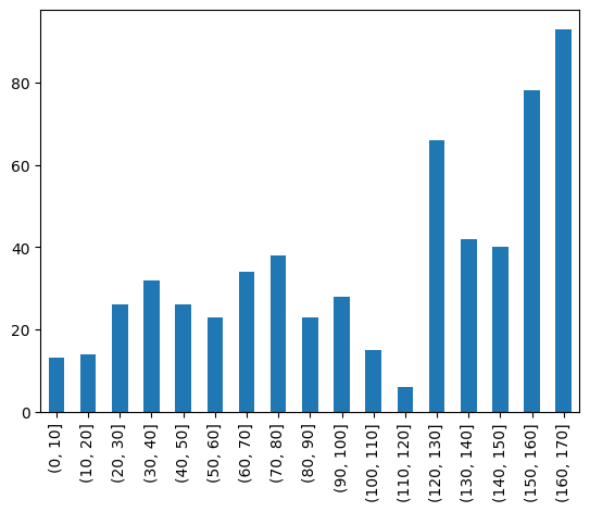
For example, let’s assume that you want to analyse the length of the different trajectories within a dataset. This may be useful for finding anomalies. In the following, we will count the number of measurements per traffic participant.
[15]:
import pandas as pd

tj_length = ds.apply(len, by="trajectory")

# create bins of width 100 measurements and count traffic participants within bins
ds_binned = pd.cut(tj_length, range(0, tj_length.max(), 100))
counts = ds_binned.value_counts().sort_index()

ax = counts.plot(kind="bar")
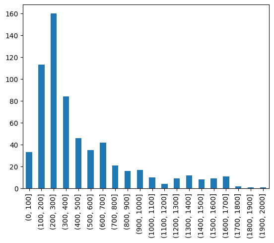
If you are instead interested in the length of each trajectory in meter, we can utilize shapely. To achieve this, we convert the tasi.TrajectoryDataset to a tasi.GeoTrajectoryDataset and gain access to the shapely feature set. This enables us to use the length attribute which is the length of the geometry.
[16]:
import numpy as np

gds = ds.as_geo("position")
tj_length = gds.length

# create bins of width 100 measurements and count traffic participants within bins
ds_binned = pd.cut(tj_length, range(0, np.int32(np.round(tj_length.max())), 10))
counts = ds_binned.value_counts().sort_index()

ax = counts.plot(kind="bar")